 Published on Sep 11, 2025 by Arcadia Science
 Efficient GFP variant design with a simple neural network ensemble
Contributors (A-Z)
Efficient GFP variant design with a simple neural network ensemble
Purpose
While machine learning has transformed protein engineering, experimental validation often lags behind. Developing generative models and laboratory capacity in parallel may help close the gap between model-based representations and biological reality. Here, we created a lightweight framework combining computational prediction with laboratory testing to design novel variants of green fluorescent protein from Aequorea victoria (avGFP).
Using a previously published large-scale deep mutational scanning (DMS) dataset, we trained an ensemble of convolutional neural networks (CNNs) to predict avGFP fluorescence across its fitness landscape. Using a random mutagenesis strategy, we generated 1,000 novel GFPs and predicted their brightness using the CNN ensemble. From these, we chose ten candidates — five predicted to be highly fluorescent and five predicted to be weak. Using a dual-reporter system (RFP–GFP fusion) in Escherichia coli, we experimentally identified brighter variants than the baseline GFP. Several others retained measurable fluorescence, though predictions didn't fully align with experimental outcomes.
This work demonstrates that in silico and experimental capacities can be spun up in parallel and inform each other, potentially allowing more effective navigation of local protein fitness landscapes. Notably, the entire pipeline — from conception to laboratory validation — was completed in under four months, establishing a framework that can be iterated on in weeks. While discrepancies between predicted and measured brightness highlight areas for improvement, the study validates the utility of combining machine learning and experimental biology for efficient protein design.
- Data from this pub, including sequence embeddings, is available on Zenodo.
- All associated code, including the CNN ensemble model, is available on GitHub.
Share your thoughts!
Feel free to provide feedback by commenting in the box at the bottom of this page or by posting about this work on social media. Please make all feedback public so other readers can benefit from the discussion.
We’ve put this effort on ice! 🧊
#ProjectComplete
This project helped us de-risk several components of iterative protein design that we’re now applying toward other, more central efforts. Given this, we’ve decided to ice further work on novel GFP design.
Learn more about the Icebox and the different reasons we ice projects.
Background and goals
Protein engineering is rapidly changing. Machine learning approaches, particularly protein language models (pLMs), continually expand the space of computationally accessible designs. pLMs are highly diverse, varying broadly in sizes, architectures, tasks, datasets, and modalities [1]. pLMs also possess great generative capacities; a single design campaign might generate tens of thousands to millions of novel sequences (e.g., [2][3]). The scale at which novel proteins can be created, and the number of tools available for doing so, is unprecedented.
Experimental validation has lagged behind the in silico design boom [4][5]. Most publications describing novel pLMs limit experimental testing to just a few proteins, if any. In many ways, this makes sense. Protein biochemistry is often slow and expensive [5]. Many proteins aren’t easily synthesized, purified, or assayed in the lab. However, the upsides of experimental validation, when possible, are manifold. Other than basic confirmation of model predictions, experimental approaches facilitate iterative design [6], disentangle function from fitness [6], and help with model fine-tuning, among other applications.
However, even if experimental approaches became easier, another bottleneck plagues protein design: navigation of fitness landscapes. While methods like deep mutational scanning (DMS) can be used to estimate fitness distributions over samples of a protein sequence space, given the combinatorial complexity of sequence possibilities and the difficulty of comprehensive sampling, doing this accurately is notoriously difficult. What’s more, fitness is rarely distributed uniformly. Fitness landscapes are defined by peaks and valleys of varying size, many of which will be invisible to any given DMS dataset. Because of this, engineering functional proteins, even within regions that are local to wild-type sequences, remains challenging.
A lightweight approach combining computational design and experimental validation might help us resolve local aspects of protein fitness through iterative exploration. Joint exploration of a protein family in the lab and in silico could help close the gap between a model-based representation and biological reality, allowing more active and intentional exploration of local design space. We focused on GFP for our initial development given its extensive characterization [7], the availability of DMS datasets [8], and its inclusion in other recent pLM-based design efforts [3]. Using an ensemble of convolutional neural networks (CNNs), we learn local aspects of the GFP fitness landscape, generate novel sequences, and experimentally validate them.
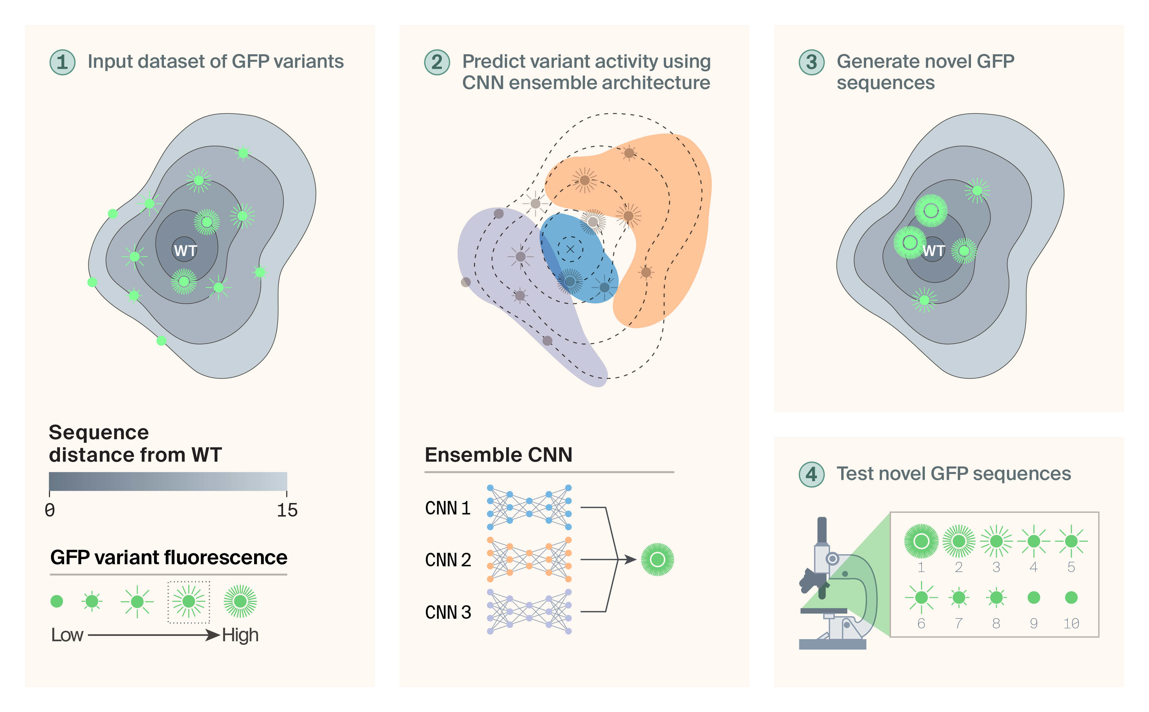
Overview of the approach.
We used variants of avGFP generated by deep mutational scanning as the starting point for our design efforts. Variants occupied various regions of the avGFP sequence space and possessed a range of fluorescence brightness values (1). We implemented an ensemble of CNNs to learn the heterogeneity of observed brightness values (2). A random mutagenesis procedure then generated novel variants and their brightness values were predicted using the ensemble CNN (3). Finally, a panel of 10 candidate proteins was experimentally tested (4).
Access our data, including sequence embeddings, on Zenodo (DOI: 10.5281/zenodo.17088257).
The approach
Data and model architecture
Data are from Sarkisyan et al.'s deep mutational scanning study of green fluorescent protein variants [9], specifically the "amino_acid_genotypes_to_brightness.tsv" file available on figshare. We converted the original indexing system by applying a +2 offset to align with wild-type amino acid positions and modified the substitution notation to follow the format <start AA><position><substituted AA>. All sequences containing stop codons ("*") were filtered from the dataset, removing 2,310 variants from the original 54,026 sequences to yield a final dataset of 51,716 GFP variants with experimentally measured fluorescence activities, where brightness scores above 2.5 correspond to visibly fluorescent proteins.
Our approach leverages ESM-2, a state-of-the-art protein language model with 15 billion parameters trained on millions of protein sequences [10]. Each GFP variant was encoded as a 5,120-dimensional vector by taking the mean representation from ESM-2's 47th layer, a choice that captures both local amino acid context and global sequence patterns. The dataset consisted of GFP variants with experimentally measured fluorescence activities from deep mutational scanning experiments [8], providing the ground truth for model training.
We developed a CNN ensemble architecture specifically designed to predict GFP variant activity from ESM-2 embeddings. The ensemble approach was motivated by recent work [11], which demonstrated that individual neural networks trained with different random initializations can exhibit significant variation when extrapolating beyond their training data, but that ensemble methods can improve robustness for protein design tasks. This study showed that simple ensembles of convolutional neural networks enable more reliable design of high-performing variants in local fitness landscapes, making them well-suited for our goal of designing GFP variants close to the baseline sequence.
Our ensemble combines multiple convolutional components, each with different architectural characteristics to maximize pattern recognition capability. The individual CNN modules use 32 channels and are designed to process the 5,120-dimensional ESM-2 vectors, treating them as structured data where spatial relationships within the embedding may correspond to functional relationships in the protein.
Training followed a consistent protocol: Adam optimizer with learning rate 1e−3, batch size 64, 100 epochs, L2 regularization (weight decay 0.01), and gradient clipping at 1.0 to ensure stable training dynamics. This configuration was chosen to balance learning efficiency with regularization, preventing overfitting to the training data.
A critical consideration in protein design is the relationship between evolutionary distance from wild type and model prediction accuracy. Our analysis of model performance across different Hamming distances revealed significant degradation in predictive power as the number of mutations increased, with models often achieving negative R² values when extrapolating to variants with substantially different mutation counts than their training data. This phenomenon motivated our focus on four-mutation variants, which represents a balance between exploring meaningful sequence space and maintaining reliable prediction accuracy.
To evaluate our models in a realistic protein design scenario, we implemented a computational pipeline to generate and screen novel GFP variants. Starting from the baseline avGFP sequence (which has an F64L substitution) [9], we systematically generated 1,000 unique variants, each containing exactly four mutations, a constraint that keeps variants in the "local neighborhood" while allowing for meaningful functional changes.
Our generation strategy was deliberately simple: random selection of four positions followed by random amino acid substitutions at those sites. While more sophisticated approaches exist (directed evolution algorithms, gradient-based optimization), this sampling method was quick and easy, allowing us to focus on building out an end-to-end feedback loop.
Quality control was essential. We filtered out any sequences already present in our training data to ensure our predictions were truly novel. The remaining 1,000 unique sequences were then processed through the ESM-2 embedding pipeline, generating the 5,120-dimensional vectors needed for activity prediction.
Experimental analysis
To test the effectiveness of our model at predicting variant activity, we selected ten proteins to generate, express, and test in the lab.
Construct design
Following Sarkisyan et al. [9], our constructs contain an N-terminal RFP followed by our avGFP variants. Between the two is a rigid, alpha-helix-rich linker (sequence: GSLAEAAAKEAAAKEAAAKAAAAS) designed to minimize Förster resonance energy transfer (FRET) [12], [9]. The non-mutated RFP allows us to normalize for varying expression levels, and its presence at the N-terminus before the GFP increases the likelihood that RFP will fold normally regardless of the effect of mutations on the fold of the GFP [9].
We synthesized ten variant GFPs and five control sequences and cloned them into a pET28a(+) expression vector between the NcoI and XhoI insertion sites (Twist Biosciences). Each sequence was codon-optimized for E. coli expression. The RFP we used was mKate [13]. For our baseline GFP, we used the avGFP F64L used by Sarkisyan et al. [9] for enhanced E. coli expression. Our selected variants are all four substitutions away from this baseline (Table 1). In addition to these variants, we also included our baseline sequence, an empty vector, and three sequences from Sarkisyan et al. [9]: the “best” or brightest variants, the protein that represents the lower edge of the “fit” distribution, and the “worst” or least-bright variant.
Name | Control/variant | Substitutions from baseline |
Baseline GFP | Control | None (apart from the F64L mutation that all of the proteins have) |
Best | Control | T37S, K40R, N104S (T36S, K39R, N103S in their data) |
Mid | Control | L14Q, Y105C, I135V, H138R (L13Q, Y104C, I134V, H137R in their data) |
Worst | Control | F26I, Q182R, K213R (F25I, Q181R, K212R in their data) |
GFP1_1 | Variant | K2L, G50E, Q175F, L194A |
GFP1_2 | Variant | T58Q, K100I, G159I, V192K |
GFP1_3 | Variant | S27I, P55D, K139W, L206I |
GFP1_4 | Variant | M0K, G3M, E141P, H230P |
GFP1_5 | Variant | T48M, K100S, E131H, K157M |
GFP1_6 | Variant | E31S, H180K, T202I, N211I |
GFP1_7 | Variant | K2Q, K100N, E114Y, G227N |
GFP1_8 | Variant | L6C, V10Y, E131I, H230L |
GFP1_9 | Variant | P57Q, I127A, T224A, L235M |
GFP1_10 | Variant | N104Q, P191G, N197M, M232W |
Table of GFP variants tested.
Proteins labelled “control” are from Sarkisyan et al. 2016 while those labelled “variant” are generated here. Positions and identities of non-baseline substitutions are provided.
Transformation and expression
We expressed all proteins in NEB T7 Express cells using the manufacturer’s protocol (NEB-C2566H). Our only deviation was splitting each 50 µL aliquot into two 25 µL aliquots. After an hour-long recovery, we plated 50 µL on LB plates with 50 µg/mL kanamycin. Like Sarkisyan et al. [9], we allowed the cells to grow overnight at 37 °C, then wrapped the plates in Parafilm and incubated them at 4 °C for 24 hours. We then picked single colonies into 15 mL of TB with 50 µg/mL kanamycin and allowed them to grow overnight. The next morning, we diluted the cultures 1:100 in 10 mL of fresh TB with kanamycin. After 3 h of growth at 25 °C, we added IPTG (isopropyl β-D-1-thiogalactopyranoside) to a final concentration of 1 mM to induce expression and then continued growth at 25 °C for the remainder of the experiments.
Plate reader assay
We used our SpectraMax iD3 plate reader to track fluorescence over time. Defining time point zero as three hours after IPTG induction, we measured brightness of both green (excitation 485 nm, emission 525 nm) and red (excitation 560 nm, emission 670 nm) fluorescence every 24 hours for seven days following induction. To limit bleeding from adjacent wells, we used black Costar plates with clear bottoms and aliquoted 200 µL from each culture each day. We added a short orbital shake before reading to disturb and resuspend any cells that may have settled.
We used measures from day two for our analyses, as there was reasonably high fluorescence for both the green and red fluorescence at this time point, and cells were healthy. To compare between samples, we normalized the GFP fluorescence by dividing the green fluorescence by the red fluorescence for each sample and averaging across replicates. Additionally, we normalized to the baseline GFP values.
This analysis can be found in this notebook on GitHub.
Microscopy
For imaging, we sealed 2 µL of cells between a coverslip and a slide. We imaged samples using a 40× 0.95 NA air objective (Nikon) mounted on an inverted Nikon Ti2-E confocal microscope fitted with an ORCA-Fusion BT digital sCMOS camera (Hamamatsu) and a LIDA Light Engine (Lumencor) for illumination controlled with NIS-Elements software (v5.42.03). We employed an NIS-Elements JOBS workflow where we imaged a 4 × 2 grid for each sample. We took images with 561 nm and 488 nm excitation. The displayed intensity range is set per channel based on a random sample of 20 images from that channel.
Code, including the CNN ensemble model, is available in our GitHub repo (DOI: 10.5281/zenodo.17088632).
Pub preparation
We used ChatGPT to help clarify and streamline text that we wrote and suggest wording ideas. We also used it to help write code and provide suggestions on our code that we selectively incorporated. We used Grammarly Business to suggest wording ideas and then chose which small phrases or sentence structure ideas to use. We also used Claude to help write code, suggest wording ideas, expand on summary text that we provided, and help copy-edit draft text to match Arcadia’s style.
The results
Generating novel GFP sequences
Like other proteins, GFP’s fitness landscape is complex. Peaks are unevenly distributed and can be steep: small numbers of random mutations can lead to total loss of fluorescence [14] (Figure 1, A). Given this heterogeneity, it’s likely that no single model will predict GFP activity over both local and global portions of the fitness landscape. Recent work has found that ensemble approaches might be more robust to the unevenness of fitness landscapes [11].
Motivated by this, we built an ensemble architecture of convolutional neural networks (CNNs) trained on an avGFP DMS dataset [9]. Our ensemble approach leverages the complementary strengths of the five constituent CNN models trained on ESM-2 embeddings (15 billion parameters) of 51,716 avGFP variants that spanned a range of Hamming distances from the baseline sequence (n mutations = 1–15) and brightness distributions (Figure 2, A). Each model was trained on a different convolutional kernel size (sizes = 5, 5, 8, 10, and 16) to allow sequence patterns across multiple scales to be captured (Figure 1, B). The ensemble CNN predicted GFP activity well up to a Hamming distance of 8 (Figure 2, B). Given the sparsity of functional proteins sampled at these greater Hamming distances and the observed distribution of avGFP brightness (Figure 2, A), we decided to focus our design efforts on four-mutation variants. At this distance, 6.74% of variants in our dataset score above baseline performance, while 54.37% remain functional (fluorescence score > 2.5). This constraint ensured we were operating within a regime where our CNN ensemble could make reliable predictions while still accessing variants with potential for improvement.
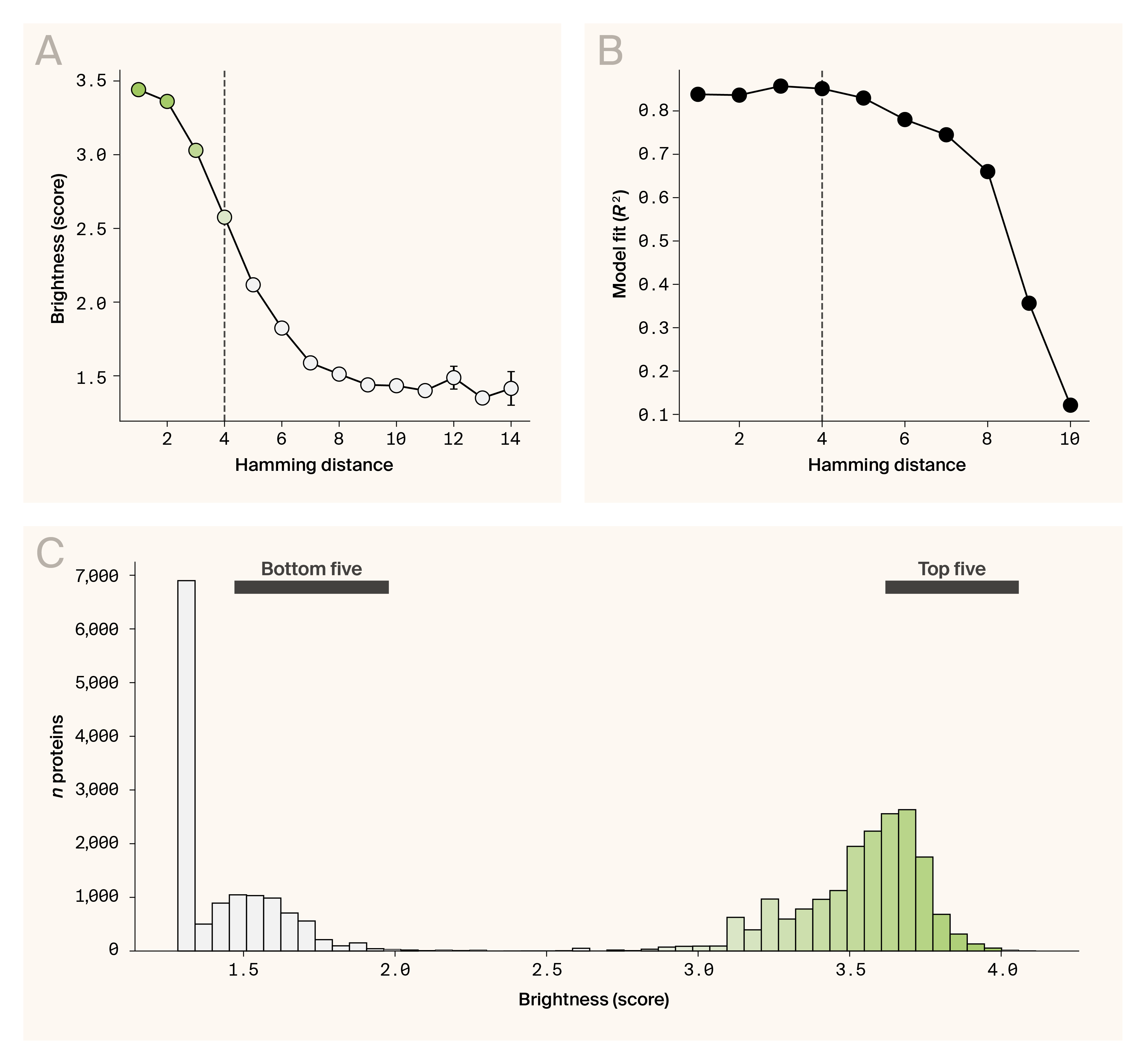
Generating novel GFP variants.
(A) Distribution of average avGFP brightness as a function of Hamming distance. A Hamming distance of four is highlighted by the dotted line.
(B) Distribution of ensemble CNN model fits (R2) as a function of Hamming distance.
(C) Distribution of the predicted brightness values as scored by the ensemble CNN. The range of brightnesses at which the top and bottom candidates used for experimental validation are indicated with labeled bars.
Our generation strategy employed random mutagenesis with uniform sampling across all 20 canonical amino acids. For each variant, we randomly selected four positions from the 238-residue baseline sequence and replaced each with a randomly chosen amino acid different from the original residue. While more sophisticated approaches exist, including structure-guided design and evolutionary-based sampling, this uniform random strategy was chosen to provide an unbiased exploration of sequence space that was quick and easy to implement.
Using this strategy, we generated 1,000 novel sequences and predicted their activities using the ensemble CNN model (see “The approach”). Predicted fluorescence scores ranged from 1.19 to 3.89, with a mean of 1.85 ± 0.66, indicating substantial predicted variation in activity across the generated variants (Figure 2, C). From the top 100 predicted sequences, we selected the top five and bottom five variants to provide a wider range of predicted activity for experimental validation (Figure 2, C).
Experimental validation
To evaluate the novel GFP sequences we generated, we used a dual-reporter system where an N-terminal RFP is fused via a rigid linker to the GFP variant of interest, similar to Sarkisyan et al. [9]. This allowed us to monitor expression of our proteins with red fluorescence, while measuring activity or fitness of our proteins with green fluorescence. Based on this setup, we were able to express all ten variants along with the controls we included, our baseline GFP, and a few proteins from the distribution of Sarkisyan et al. (best, mid, worst) [9]. Our analysis differed from Sarkisyan et al. in that they employed cell sorting while we looked at individual cell populations using a plate reader or microscope [9].
While all proteins did consistently display red fluorescence, their level of green fluorescence intensity, or fitness, was more varied (Figure 3, A). First, the controls we selected from the Sarkisyan et al. dataset aligned well with the expected, with the “best” protein appearing brightest, the “worst” protein being the dimmest, and the “mid” protein being somewhere in the middle [9] (Figure 3, B). Inconsistent with their results, we found that our baseline GFP was brighter than the “best” protein variant from their dataset (Figure 3, B).
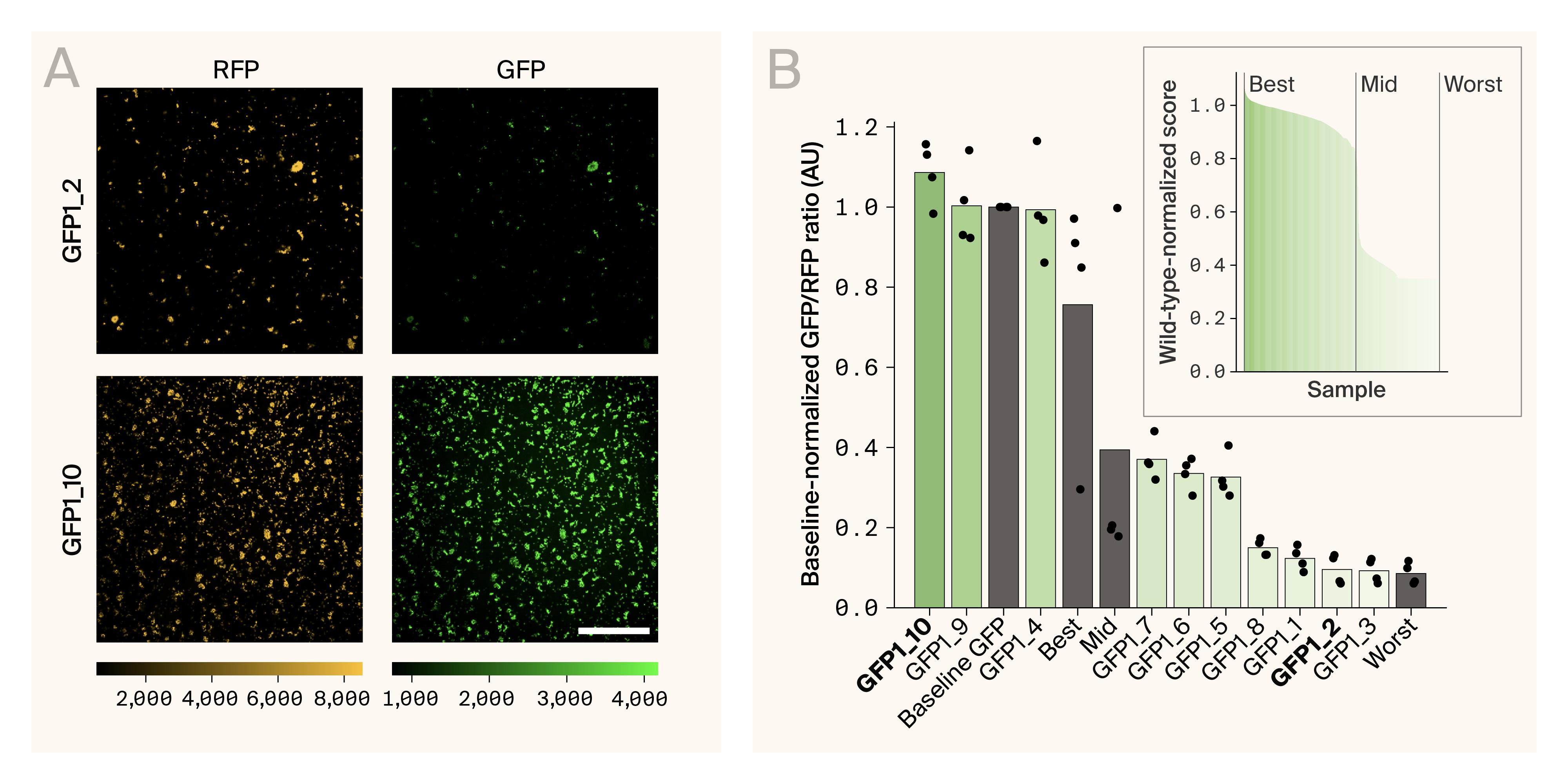
Experimental analysis of GFP variants reveals functional proteins.
(A) Fluorescence microscopy images of two variants, GFP1_2 and GFP1_10. GFP1_10 was our brightest variant, while GFP1_2 was one of the dimmest. The left and right images show the same field of view with RFP fluorescence on the left and GFP fluorescence on the right. Scale bar is 100 µm.
(B) The baseline-normalized GFP-to-RFP ratio for the ten variants and the three controls, along with the baseline. The bars show the mean, while the dots show individual replicates. The inset is the baseline-normalized brightness “score” values from the training data, highlighting where the controls fall within that data.
From our variants, we found three that were as bright or brighter than our baseline GFP and the “best” protein control, variants 10, 9, and 4 (Figure 3, A & B). Two of these are from the “bottom five” and one is from the “top five” (Figure 2, C). Three of our proteins were around the “mid” controls (Figure 3, B). These were fluorescent, but not as bright as the baseline GFP. Finally, four proteins were very weakly fluorescent and underneath the threshold that Sarkisyan et al. defined as fluorescent in their analysis, variants 8, 1, 2, and 3 [9] (Figure 3, A & B). Interestingly, this includes the three proteins from the “top five” set (Figure 2, C).
Access our data, including sequence embeddings, on Zenodo (DOI: 10.5281/zenodo.17088257).
Key takeaways
Among the most common bottlenecks that limit protein design are the difficulty of experimental validation and incomplete understanding of fitness landscapes (the space of functional outcomes given possible sequences). We hypothesized that, by developing computational prediction and experimental validation capacities in parallel, these bottlenecks could be addressed in tandem. Using avGFP as our test case, we trained an ensemble CNN model that could accurately predict protein brightness up to eight mutations away from the baseline protein. At the same time, we generated an approach to experimentally validate GFP brightness using a dual-reporter system. Of 10 novel GFP variants, we identified two that were brighter than the baseline, while several others displayed fluorescence. Interestingly, despite predicting multiple functional proteins, the ensemble CNN, as implemented, failed to accurately predict the distribution of measured brightnesses, highlighting a clear target for potential future development. Finally, it should be noted that this body of work — from conception to validation — was completed in under four months and can now be iterated over on the order of weeks.
Next steps
This work was central to creating an internal approach to jointly developing computational and experimental protein design capabilities. The lessons learned and tools generated here have already been applied to other efforts more central to our goals. Given this, we have decided to ice these efforts and forego any future iteration on GFP design.
That said, there are several next steps we'd suggest to those interested in continuing this work. Resolving the mismatch between predicted and empirical brightnesses would be worth it. From an experimental perspective, testing more variants may help connect specific residues/sequences to brightness variation and resolve this disconnect. Computationally, it might be useful to implement more sophisticated procedures for protein generation. Given the well-known constraints around GFP’s active site and other structural features, structurally informed approaches might be a sensible next step. It would also be interesting to further fine-tune the two variants that were brighter than the baseline GFP. Our framework could be used to perform simple in silico directed evolution of these variants and, in the process, further map the complexities of GFP’s local fitness neighborhood.
References
Share your thoughts!
Feel free to provide feedback by commenting in the box at the bottom of this page or by posting about this work on social media. Please make all feedback public so other readers can benefit from the discussion.
