 Published on Jun 16, 2025 by Arcadia Science
 Epistasis and deep learning in quantitative genetics
Contributors (A-Z)
Epistasis and deep learning in quantitative genetics
Purpose
Deep learning (DL) methods are becoming increasingly common in biological research. While powerful in some contexts, it's often unclear what biological patterns DL models end up learning and how much of an advantage they provide over simpler alternatives. Such questions can be probed most efficiently in highly distilled, simulated datasets, providing insight into the underlying behavior of DL models. Here we tackle this task in the context of epistatic interactions in genotype-to-phenotype mapping. We test the ability of a multilayer-perception (MLP) to beat conventional linear regression in three in silico experiments meant to probe the behaviour of DL across familiar quantitative genetics parameters space, namely numbers of QTLs, relative genetic variance components, and genetic correlations/pleiotropy among phenotypes. Our results help give us intuition about when and where applying DL is most likely to result in success in more complex, real-world biological datasets.
- Data from this pub is available on Zenodo.
- All associated code is available in this GitHub repository.
Share your thoughts!
Feel free to provide feedback by commenting in the box at the bottom of this page or by posting about this work on social media. Please make all feedback public so other readers can benefit from the discussion.
Background and goals
In recent years, deep learning (DL) has seen widespread adoption in biological applications, from predicting gene expression and variant pathogenicity to capturing the “language” of protein sequences [1][2][3]. It’s becoming clear that, in some cases, DL can outperform simpler statistical models. However, the reason for the success of DL in biological applications is often less obvious. Predicting when and where applying DL provides real benefits remains hard, especially in cases where the underlying biological questions being modelled are poorly understood.
In this pub, we explore the utility of DL for one specific biological application, modelling genotype–phenotype relationships. Conventional methods for mapping genotype to phenotype based on linear regression have proven useful in a swath of biological applications, from understanding and treating disease [4], to increasing the efficiency of agricultural breeding [5], and understanding evolution [6]. Consequently, DL has increasingly been applied to such genotype–phenotype mapping tasks. Some of these efforts have resulted in significant improvements in genotype–phenotype prediction accuracy (relative to linear regression), although results tend to be phenotype and dataset-specific [7][8][9][10]. A significant number of studies, however, report little apparent benefit to applying DL at all, if not a detriment [11][12][11][13][14][15]. Conveniently, the framework of quantitative genetics allows us to make predictions about which phenotypic variance components DL models should be capturing that linear models aren't, which provides a useful baseline for assessing the behaviour of DL in this setting. Chief among these are nonlinear interactions that linear models will miss, such as epistasis and genotype by environment effects.
Epistatic interactions are perhaps the most poorly explored component of genotype-to-phenotype maps. Most quantitative geneticists ignore epistasis. This might make sense for certain study systems, for example, in human-like populations, most phenotypic variation should be explainable by additive effects [16]. However, additive effects can capture all manner of biological effects, converting biological epistasis to statistical additivity [17]. Under the right conditions, a significant component of phenotypic variance can be decomposed into statistical epistatic variance even under the conventional quantitative genetics statistical framework [18]. This is consistent with a vast array of studies on protein function, where beyond a handful of substitutions, epistatic interactions become the dominant determinant of protein fitness (e.g., see [19]). In short, it's almost certain that epistasis is a major driver of phenotypic variation across the tree of life [20]. Building models geared towards capturing epistatic effects is a critical step in building a fundamental understanding of genotype–phenotype mappings.
The scattered array of results and efforts on applying DL to genotype–phenotype mapping inspired us to ask a simple question: Can we understand when and where DL models outperform linear regression in a G→P context? We point this question towards the problem of capturing epistasis. Our aim isn't biologically realistic simulation per se. Rather, we use simplified datasets to probe the basic behaviour of DL models with regard to being able to capture epistatic variance under conditions where we know epistasis is statistically apparent. Our results illustrate the parameter space under which DL models can capture epistasis in the convenient units of classical quantitative genetics (relative variance components, numbers of QTLs, numbers of samples, etc.).
Access our simulated data on Zenodo (DOI: 10.5281/zenodo.15644565).
The approach
Scaling experiment
Simulations
For our initial set of simulations probing the scaling behaviour of DL models, we did a parameter sweep across 1) log-scaled number of simulated samples (from 103–106 individuals) and 2) Number of causal QTLs (16–6,326 bi-allelic loci). We tested each sample size parameter with 10 causal QTL number parameters. We chose these QTL numbers based on a scaling factor relating the number of possible pairwise QTL interactions to the number of samples, defined by equation 1 below. A scaling of one implies as many samples as possible pairs of QTLs, a scaling of 0.1 implies 10× as many samples as possible pairs of QTLs, a scaling of 10 implies 1/10 as many samples as possible pairs, and so on:
We tested the following 10 scaling factors (0.1, 0.2, 0.3, 0.5, 1, 2, 4, 7, 12, 20), generating datasets across both n > p and p < n regimes (with regard to numbers of epistatic pairs). The actual number of QTLs used to achieve these scaling factors was calculated using the following formula, rounding the output to the nearest even integer:
This scaling provides a convenient way of generating combinations of sample size and QTL numbers that probe informative and comparable parameter spaces across simulations.
We used AlphaSimR (v1.61) to generate all simulated genotype–phenotype datasets. By altering the relAA parameter in the addTraitAE function, we generated five independent phenotypes in each simulation run, ranging from purely additive to almost fully epistatic (relAA values: 0, 0.1, 0.5, 1, 3). This, in practice, resulted in a set of traits that had the following relative additive variance (VA/VG) components: 1, 0.8, 0.5, 0.3, 0.15. For simplicity, all phenotypes were scaled to have a mean of 0 and a variance of 1, and had a broad sense heritability of ~0.99. We simulated haploid populations with no genetic or demographic structure. Founder genomes were sampled using the quickHaplo function, which generates a population with roughly 50/50 allele frequencies (based on simple binomial sampling) and loci that are random with respect to each other (i.e., no linkage disequilibrium). We then directly used the genotypes and phenotypes of these founders for genomic prediction with no further manipulation. We generated 10 replicates of the 103–104 sample simulations, five replicates of the 105 sample simulations, and three replicates of the 106 sample simulations, decreasing replicates in the larger simulations due to increasing model fit times and reduced variability between simulation replicates.
Model fitting
We used two methods to fit linear regression models to provide a performance baseline for more complex DL models. First, we used the RidgeCV model implemented in scikit-learn (v1.5.1) to fit a ridge-regression model on each phenotype independently. To evaluate model performance in a robust way, we randomly split the data in a 15%–85% test-train split, determined the best tuning parameter 𝛌 through cross-validation, performed model fitting, and finally calculated Pearson's r on predicted vs. true phenotypes in the test data subset. We repeated this process 10 times, taking the average Pearson’s r as the final model performance metric. This approach is statistically analogous to performing rrBLUP, a classic genomic prediction model framework used in the field of plant and animal breeding, where 𝛌 is set analytically through variance component decomposition.
While analytically fit penalized regression is the most obvious benchmark to use for DL models, this family of models becomes hard to work with when sample sizes and parameter numbers become large due to quadratically increasing computational complexity. To manage this, we fit an approximation of ridge regression using stochastic gradient descent. Briefly, we implemented a simple model with one linear layer in PyTorch (v1.5.1) with a custom loss function consisting primarily of a mean absolute error (MAE) loss, but with a Kullback–Leibler (KL) divergence component, constraining the distribution of weights in the linear layer to match a prior based on the normal distribution N(0,1). The KL divergence was computed as 0.5 × sum(weights2) across all model parameters. The total loss then was a sum of these two components, where we weighted the contribution of the KL divergence term through a tunable parameter set to 0.1. We fit the model using stochastic gradient descent (learning rate 0.1) with the PyTorch ReduceLROnPlateau scheduler that halved the learning rate after three epochs without improvement in the validation loss. To prevent overfitting, we implemented early stopping with a patience of 20 epochs and a minimum improvement threshold of 0.001 on the validation loss. We found high concordance in the performance of the stochastically fit linear model and the RidgeCV models we fit on smaller datasets (103–104 samples) using a KL divergence loss weight of 0.1 (see analysis in this supplementary notebook). As a result, we used this stochastically fit linear model as the baseline for simulation runs across all our parameters.
Our deep learning model was constructed as a two-hidden-layer multilayer perceptron (MLP) network. While this is a relatively simple architecture, MLPs can approximate any function (linear or nonlinear) [21], making them amenable to learning epistatic interactions, and fully connected feed-forward layers such as the ones we employ are an essential component of many, more tailored DL models such as convolutional neural networks and transformers [22][23]. We implemented the MLP model in PyTorch (v1.5.1), with an architecture consisting of an input layer of size 2 × QTLn (one per one-hot encoded QTL), followed by two hidden layers of size 4,096. After each hidden layer, we applied batch normalization (with momentum parameter 0.8) followed by leaky ReLU activation functions (negative slope 0.01). The output layer contained five units (one per phenotype) with a linear activation function.
MLP training was performed with a batch size of 128 on an 85%–15% train-test data split (the same split as for the linear stochastically fit models). We employed a learning rate scheduling strategy using the PyTorch ReduceLROnPlateau scheduler that halved the learning rate after three consecutive epochs without improvement in the validation loss. For model training, we used the AdamW optimizer with an initial learning rate of 0.01 and a weight decay coefficient of 1 × 10⁻⁵ to mitigate overfitting. We implemented an early stopping protocol that terminated training when the validation loss failed to improve by at least 0.003 for 10 consecutive epochs, with an upper limit of 150 epochs. We used a standard MAE loss term and evaluated final model performance on the test set, reporting the Pearson correlation coefficient between predicted and actual phenotypes as for the linear regression models. We initially experimented with hyperparameter optimization for learning rate and hidden layer size values, but found negligible effects on model performance across our simulation parameters.
QTL “dilution” experiment
Our first follow-up experiment involved “diluting” a set of informative QTLs with progressively increasing numbers of uninformative QTLs to test whether DL models could still recover epistatic mappings when only a subset of loci is causal. We focused on the 104-sample scenario, as this was a large enough sample size to give reasonably consistent simulation outputs but small enough to allow for rapid model fitting and evaluation.
Simulations
As a control scenario, we chose 100 causal QTLs, a parameter space where 104 samples provide enough data for a neural network to almost fully learn the G→P map without overfitting. To these causal QTLs, we added 0, 150, 400, 650, 900, 2,400, 4,900, and 9,900 uninformative QTLs by manipulating the total number of markers sampled when creating population founders, but retaining only 100 QTLs with phenotypic effects. We only focused on epistatic traits with relAA set to 0.5 (corresponding to a VA/VG = 0.3) along with a purely additive trait (relAA=0, VA/VG = 1) as a control. We generated five replicates of each simulation condition.
Model fitting
As a first pass, we used the same RidgeCV model (implemented in scikit-learn) and MLP (implemented in Pytorch) we used in the scaling experiment to compare linear and DL model performance. The only modification to the training workflow was an additional learning rate optimization step implemented in Optuna (v3.5.0) for the MLP model. These analyses revealed the need to perform feature selection to improve model performance when many uninformative QTLs are present.
Our simple approach to implementing this first trained a modified stochastically fit linear model with a Laplace prior on the weights (approximating LASSO rather than ridge regression) to enforce more sparsity in the linear layer weights, thereby providing a simple way of extracting informative features (one-hot encoded QTLs in our case). We used the same strategy of modifying the MAE loss with a KL divergence term, using a weight of 0.001, keeping all other parameters unchanged. Selected features exceeding an importance threshold (0.03) were retained and sorted by learned weight. We then used hyperparameter optimization to simultaneously determine the optimal number of features to retain and tune the learning rate [again implemented through Optuna (v3.5.0) with 20 trials] based on validation loss in the MLP.
The final best feature set was then used to train two models: a pruned version of the LASSO model and a pruned version of the MLP. Model performance was again evaluated using Pearson's correlation between predicted and actual phenotypes in the test data.
Genetic correlation experiment
Our second follow-up experiment involved testing how much model performance can be improved when multiple genetically correlated traits are generated again using the 104-sample scenario from the initial scaling experiment.
Simulations
We generated groups of traits with pleiotropic QTLs, varying the strength of pleiotropy to generate groups of traits with varying strength of genetic correlation. We again implemented this using the addTraitAE function in AlphaSimR by specifying a cross-phenotype covariance matrix for both additive and epistatic QTL effects (using the same covariance values for both effect types). We generated phenotype sets with QTL effect covariance values of 0.25, 0.5, 0.75, and 0.95 for sets of both 10 and 100 phenotypes. Additionally, we created a control case of no pleiotropy/genetic correlation by simply creating sets of randomly initialized traits through a for-loop. We varied the number of causal QTLs from 100 to 1,000 to test if cross-phenotype genetic correlations would allow models to learn effect sizes from more QTLs than is possible for independent traits. Again, we only focused on epistatic traits with relAA set to 0.5 (corresponding to a VA/VG of 0.3) in a population of 104 samples. We generated five replicates of each simulation condition.
Model fitting
For this experiment, we used the same cross-validated ridge regression and MLP described in the previous experiments. We used Optuna to optimize the MLP's learning rate through 10 trials, leaving all other hyperparameters as is. Model performance was again evaluated using Pearson's correlation between predicted and actual phenotypes in the test data.
Code, including all scripts necessary to reproduce our simulated data and analyses, is available in our GitHub repo (DOI: 10.5281/zenodo.15659065).
Additional methods
We used Grammarly Business to help copyedit draft text to match Arcadia’s style. We used Claude to help write code, review code, streamline and clarify text that we wrote, and suggest relevant literature that we further reviewed and cited. We also used ChatGPT to help find information during code review. We used arcadia-pycolor (v0.6.2) [24] to generate figures before manual adjustment.
The results
We performed three simple in silico experiments to probe the ability of DL models to capture patterns of statistical epistasis in genotype-to-phenotype prediction tasks. The first "scaling" experiment establishes the baseline data requirements for DL models to capture statistical epistasis across phenotypes of varying complexity. The second "dilution" experiment tests how these scaling patterns change when causal QTLs are mixed with uninformative ones, simulating more realistic genomic data. The third "genetic correlation" experiment explores whether training on multiple correlated phenotypes further alters the scaling behavior, adding one final dimension of biological realism.
DL scaling experiment
In our first “scaling” experiment, we probed the most basic aspect of scaling one can study in a G→P mapping context: How much data does a DL model need before it starts outperforming a linear regression benchmark? The answer helps establish a baseline for when we expect DL models to capture statistical epistasis. It also starts to give us insight into why DL models fail to provide an advantage in some G→P datasets but not in others.
We tested model performance across a range of phenotype genetic architectures, from purely additive (VA/VG = 1) to almost fully epistatic (VA/VG = 0.15). Causal QTL number was chosen by adjusting for the number of possible epistatic QTL pairs. We focused on pairwise interactions rather than additive terms, since the former grows much faster than the latter as QTL number increases. Our parameter selection strategy involved sampling set ratios of possible QTL pairs to sample sizes, starting at 0.1× as many QTL pairs as samples, and finishing with 20 times as many QTL pairs as samples (see “The approach” for more details).

Scaling performance of a multilayer perceptron (MLP) in the context of simulated genotype to phenotype prediction.
Results shown for five phenotypes, ranging from purely additive (VA/VG = 1) to mostly epistatic (VA/VG = 0.15), across four dataset sample sizes (103–106), and various causal QTL numbers (see methods).
(A) Relative test set prediction gain of MLP against a linear regression benchmark vs. QTL number. Y-axis statistic calculated as the difference in Pearson’s r between two models normalized by the linear model's Pearson’s r. Dashed line indicates model parity.
(B) Test set Pearson’s r for MLP only, plotted against scaled number of QTLs. Scaling calculated as number of possible pairwise QTL interactions divided by sample size. Dashed line indicates parity between sample size and number of possible epistatic interactions.
The DL model scaled in a surprisingly consistent fashion relative to the linear benchmark. Regardless of sample size and trait architecture, the DL model tended to exhibit two stable regimes. At small QTL numbers (QTL pairs ≪ sample size), the DL model learned to predict almost all epistatic and additive variance, outperforming the linear benchmark. At large QTL numbers (QTL pairs > sample size), the DL model shifted to learning additive effects only, approximating the performance of the linear benchmark (Figure 1, A & B). Our results suggest a fairly simple rule of thumb: our DL model starts to capture epistatic variance when there are at least 20% as many training samples as possible QTL pairs (Figure 1, B). However, predictive performance improves rapidly after this point, and most epistatic variance is explained only when there are more training samples than epistatic features to learn. Our results are considerably more variable across replicates from smaller sample sizes (particularly at 103 samples), but averaged across replicates, behaviour is consistent across all sample sizes.
On the one hand, these results are somewhat encouraging. Even under n = p conditions (with p referencing epistatic features rather than QTLs), DL can capture epistatic variance — a regime where a linear model incorporating all pairwise combinations might be theoretically solvable with regularization but would incur large computational costs. On the other hand, given the number of genotyped QTLs vs. the number of samples in most G→P mapping datasets, it's likely that in most cases DL models won’t provide a large difference in predictive power over a linear regression. However, the setup we use is, of course, artificially distilled. All the QTLs we simulate are causal, and we use a limited number of unrelated phenotypes, two conditions that are rarely true in real-world G→P datasets. Given this, we wondered what would happen if we relaxed these constraints to create more biologically realistic scenarios.
QTL dilution experiment
In the above experiment, all QTLs we simulated were informative. What happens to scaling relationships if we introduce uninformative ones? We reasoned that this “dilution” experiment would better reflect the structure of real phenotypes, which are often only impacted by a fraction of the genome. This lets us test how scaling behaviour can be managed in the case where we know some of the input data can be ablated with little loss of information. Consequently, this experiment aims to expand the parameter space where we expect DL models to outperform linear regression.
We focused on the base case of 104 samples, 100 causal QTLs, one fully additive trait (VA/VG = 1), and one highly epistatic trait (VA/VG = 0.3). From our first scaling experiment, we know that these parameters should allow a DL model to almost fully capture all variance components of these phenotypes (scaling factor of ~0.5). We progressively dilute these 100 causal QTLs with more and more uninformative QTLs (from 0 to 9,900, resulting in 100–10,000 total QTLs) to mimic the basic structure of many biological datasets where only a small subset of QTLs have large additive effect sizes (and therefore are able to contribute substantially to epistatic variance).

Performance of three genotype–phenotype models in predicting phenotypes with progressively diluted causal QTLs.
Phenotype architecture always has 100 causal QTLs, starting with no additional QTLs, and ending with 9,900 non-causal QTLs. Total QTL number for phenotypes reported on top of each subplot. Two phenotypes simulated per condition, one purely additive (VA/VG = 1), one mostly epistatic (VA/VG = 0.15). Three models are compared: a simple MLP, a pruned Lasso regression model with low-weight features removed, and a pruned MLP also trained on the same filtered features as the Lasso model. Y-axis statistic is the difference in test set Pearson’s r compared to a ridge regression benchmark, dashed line indicates model parity.
As a first pass, we compared an unmodified version of the MLP from our scaling experiment and cross-validated ridge regression on these QTL dilution datasets. We found that DL models rapidly lost the ability to capture epistatic variance as uninformative QTLs were added to the dataset (Figure 2). For the epistatic trait, DL model performance worsened with 250 total QTLs, and effectively matched the linear model at 750 QTLs and beyond. This indicated that, even though added QTLs were uninformative, the unmodified DL model wasn't able to efficiently recover biological signal to learn epistatic interactions. For the additive trait, both models were roughly equivalent up until very large numbers of QTLs (10,000), where the linear model started to outperform the DL model. While model performance did degrade rapidly with QTL number, relative to the initial scaling experiment, the DL model continued outperforming the linear model in a larger parameter space. For example, at 500 QTLs, the DL model was still demonstrating consistent benefit over the linear model. This scenario has a scaling factor of ~12.5, which is much larger than the minimum scaling factor of five identified in the first experiment.
Our results from the first scaling experiment strongly suggest that the datasets we're simulating here should be sufficient for the DL model to learn all relevant biological features (i.e., additive and epistatic effects of the causal QTLs). It follows then that if we're able to bias the attention of the model to the relevant QTLs, we may be able to recover even more epistatic variance. We experimented with several different strategies for doing so, including adding an informational bottleneck in the first layer of the DL model by reducing the number of neurons, iteratively pruning weak connections in the first layer of the DL model, and iteratively training a LASSO regression model with feature selection based on weight values. In the end, the simple strategy that we found to work most consistently involved pretraining a LASSO regression model once on all QTLs to determine feature importance (ranking QTLs by learned weight), and then using Optuna to determine the number of features to prune from the dataset based on DL test set performance with various QTL number cutoffs.
Pruning uninformative QTLs improved epistatic trait prediction for both linear and DL models in simulation replicates with 750 or more QTLs. This illustrates the overall benefits of input filtering through feature selection for any type of model (Figure 2). Compared to the pruned linear model, the pruned DL model showed evidence of superior performance for epistatic traits at intermediate QTL numbers (750–1,000), suggesting that some (but not all) epistatic variance can be recovered from a subset of informative QTLs using feature selection. However, at very large QTL numbers (> 5,000), there was no appreciable difference between the pruned linear and DL models, indicating that our strategy likely doesn't scale well as the number of uninformative markers approaches the sample size. Despite this, the pruning strategy further pushes the parameter space where a DL model can outperform linear regression to an impressive scaling factor of ~50, an almost 10× improvement over the first scaling experiment.
These results demonstrate that DL models might be able to capture epistasis when trained on more QTLs than our first scaling experiment suggested. This is particularly true if the training data are enriched for informative QTLs. However, there's another major source of statistical power that might alter the scaling behaviour of DL models: genetic correlations between multiple phenotypes. In the next experiment, we test how such a scenario might further alter DL model scaling behavior.
Genetic correlation experiment
In our third “genetic correlation” experiment, we probed how the scaling relationship between QTL number and sample size changes when models are trained on multiple genetically correlated phenotypes. This experiment injects a new axis of biological realism into our scaling tests; that organismal phenotypes aren't random with respect to each other due to pleiotropy at causal QTLs.
We again focused on the base case of 104 samples and 100 causal QTLs, simulating only epistatic traits (VA/VG = 0.3). We varied the strength of genetic correlation among these traits by adjusting the pleiotropic correlation of causal QTL effect sizes (for both additive and epistatic effects), ranging the strength of correlation from 0 (independent phenotypes) to 0.95 (almost perfect phenotypic correlation). We tested if having 10 or 100 correlated traits allowed our DL model to capture epistatic variance at larger QTL numbers (200–1,000) than possible for pleiotropically uncorrelated phenotypes.
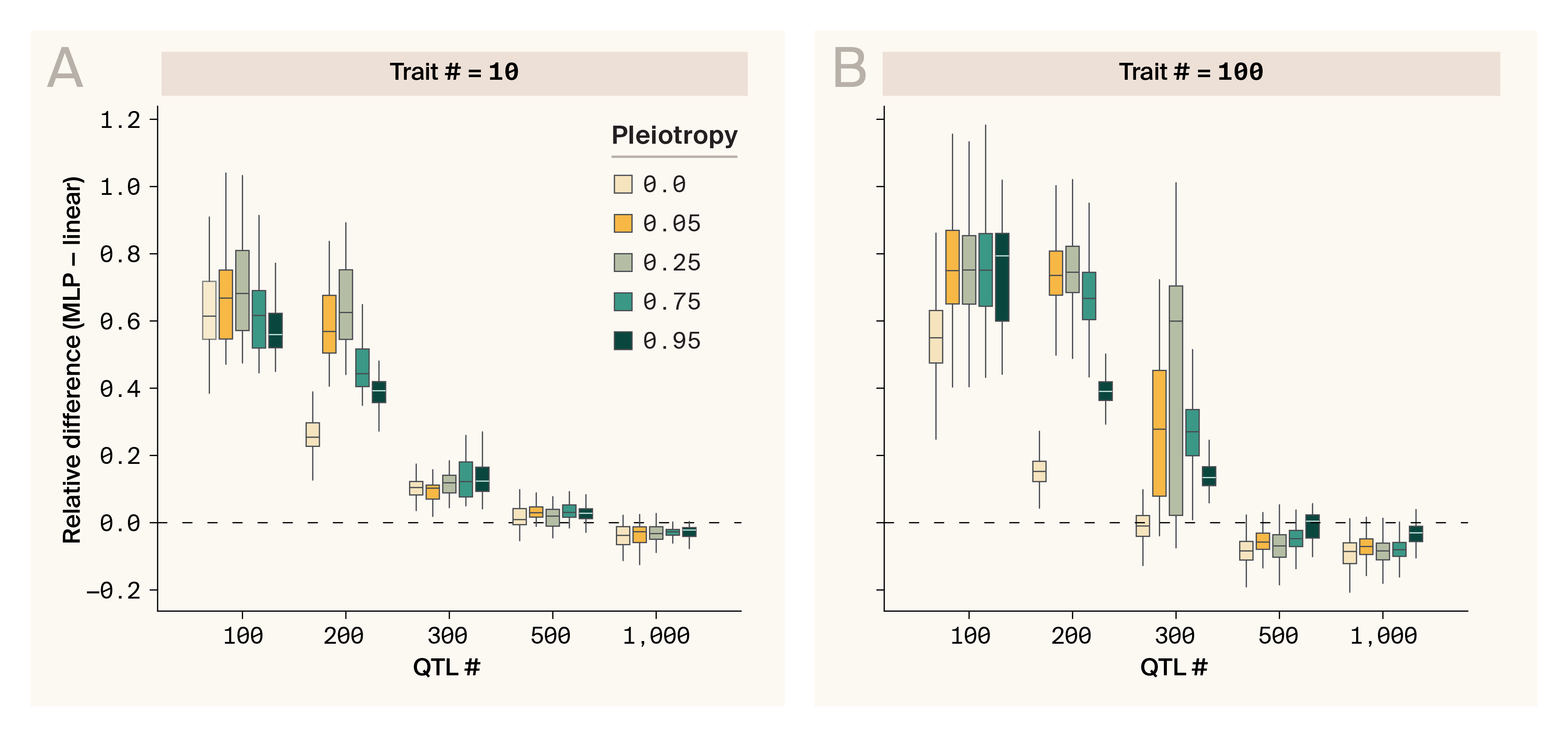
Effect of genetic correlations among phenotypes for MLP prediction performance relative to a linear model benchmark.
Epistatic phenotypes simulated (VA/VG = 0.15) with progressively larger numbers of causal QTLs (x-axis). Phenotypes range from independent (pleiotropy in QTL effect sizes = 0) to almost perfectly correlated (pleiotropy in QTL effect sizes = 0.95). Y-axis statistic is the difference in test set Pearson’s r compared to a ridge regression benchmark averaged across all phenotypes in every simulation replicate. Dashed line indicates model parity.
(A) 10 correlated phenotypes simulated.
(B) 100 correlated phenotypes simulated.
We found that multi-task learning on genetically correlated traits could indeed aid DL models in learning to capture epistatic variance. However, the magnitude of this benefit was sensitive to QTL number and number of phenotypes. In almost all cases, we found that the DL model outperformed ridge regression for phenotypes with 300 QTLs or fewer, indicating that in these scenarios the model was able to learn to recover some signal of epistasis (Figure 3, A & B), echoing results from our scaling experiment.
When examining scenarios with few QTLs, we observed that, peculiarly, DL models performed better with low levels of genetic correlation (0.05–0.25) between traits. However, this effect is likely an artifact of our simulation design rather than a biologically meaningful pattern. This happens because our simulation framework had to distribute correlated effects across a limited number of QTLs for many traits, creating an unusual information structure. In the low correlation settings (e.g., 0.05), if a QTL strongly affected one trait, it would typically have minimal effect on other traits — a pattern that becomes more pronounced with fewer QTLs and more traits. This artificial pattern diminishes in scenarios with more QTLs and fewer traits. While these nonlinear relationships aren't detected by simple linear models, our DL model could exploit this hidden structure. To address this issue, our control condition used independently generated traits rather than traits with pre-specified correlation structures. Since this pattern is a simulation artifact rather than a biological insight, we focus our interpretation on the general difference between conditions with and without genetic correlation between traits.
For both 10-trait and 100-trait simulations, pleiotropy appeared to boost DL model performance modestly only for small numbers of QTLS (100–300) with rapidly diminishing returns (Figure 3, A & B). For large numbers of QTLs (500–1,000), it appears yet again that the DL model switches to capturing additive effects, leading to overall slightly subpar performance relative to the linear benchmark, with pleiotropy only providing a minor benefit in the 100-trait simulations. The primary benefit of multi-task learning in this setting seems to be a boost in model performance when it's in a parameter space where it would be capturing epistatic variance, even on a single trait, rather than a wholesale shift in scaling relationships, as in our dilution experiment.
Focusing on the simulations with 300–1,000 QTLs and 10 traits, where pleiotropy seems to benefit DL model performance but the statistical artifact we pointed out earlier seems minimal, we note that even moderate levels of pleiotropic genetic correlation (e.g., 0.25) appear to enhance prediction accuracy. This is an encouraging result, as it suggests that multi-task learning on even moderately genetically correlated phenotypes is a fruitful approach for enhancing DL model success. This echoes our previous work with phenotype–phenotype autoencoders [25], and further reinforces our suggestion to take advantage of phenotypic mutual information. The benefits of multi-task learning have been well established in the machine learning literature [26][27], and have been shown to help in a genomic prediction context for both linear regression [28] and deep learning [8]. Consequently, a thorough examination of the strategy for which and how many phenotypes to gather data on when designing experiments will be helpful for gaining as much performance as possible from DL models aimed at capturing epistasis.
Access our simulated data on Zenodo (DOI: 10.5281/zenodo.15644565).
Key takeaways
Our in silico experiments demonstrate that deep learning (DL) models can capture complex genetic interactions (epistasis) that traditional linear models miss, but only under specific conditions. We found that DL models begin to learn epistatic interactions when training samples reach at least 20% of the possible pairwise genetic interactions, with rapid improvement as more training data was added. However, these scaling relationships are more permissive when only a subset of genetic markers are causal — a common scenario in real-world biological data. Strategic feature selection and analyzing multiple related traits simultaneously can be used to further boost model performance. These findings help us understand why DL has shown mixed results in genomic prediction tasks. They also provide practical guidelines for when to use DL. Studies considering multiple related phenotypes, populations with genetic structure, and adequate sample sizes are most likely to benefit.
Next steps
Our results have several implications for using DL models in genotype-to-phenotype mapping tasks. First, our scaling data across all experiments imply that efforts to apply DL to n ≪ p datasets (treating all possible epistatic interactions as p) will be challenging. DL will likely only provide a benefit in datasets with very large sample sizes if substantial statistical epistatic variance is present in the phenotypes of interest. Our dilution results highlight the value of constraining the training data for model performance. Conventional wisdom in fields like breeding is to use all available markers, as regularized linear models generally perform well for phenotypic prediction in n > p regimes [29][30] and this strategy allows for fine-scale tagging of haplotypic structure. However, if we're interested in using DL models to capture epistatic interactions, such a strategy fails as the number of interactions among input QTLs scales roughly exponentially. Consequently, DL models seem to benefit when constraints can be placed on their search space.
For example, convolution has proven to be remarkably effective in the field of computer vision, as it guides DL models to learn features by first looking at the local informational context in images before scaling upwards to longer-range, more abstract patterns [23][31]. Our results highlight that the key problem is figuring out how we can apply such search space constraints in the context of biological G–P mapping. An obvious first step is the one we have employed in our dilution experiment: only use informative QTLs when training a model. Another existing strategy that's often employed in the genomic prediction DL literature is to use convolution across neighboring loci to capture and summarize local LD, thereby reducing the number of input features for downstream model use [10][13][9][14]. This may be valid for achieving constraint with one major caveat from the perspective of epistasis. Epistasis manifests as the interaction between two (or more) loci. As a result, any noise with regard to genotypic state at the interacting loci will be especially harmful for prediction accuracy (as error will be compounded across multiple loci). Consequently, it’s unclear a priori if convolution, which will tend to smooth out individual genotypic signals across a chromosomal window, will always be the best approach for reducing the number of learnable features. In some cases, LD may be strong enough in a local window that convolution reduces dimensionality without much penalty on recovering epistasis, but future simulations will be needed to determine when this is the case.
One complementary strategy for inducing informative limits in the search space of DL model training would be to inject biologically informed constraints into model training. Several previous studies have attempted this through means such as encoding protein–protein interactions using graph neural networks [32] or embedding of KEGG pathways in MLP models [33]. More work, however, will be needed to evaluate which databases of biological interaction are most useful in guiding DL model training relative to standard regularized linear model baselines.
Given our findings, which G→P datasets do we expect to be well-suited to DL model training? Datasets such as F1 QTL mapping populations are probably the best suited for such tasks. While the number of polymorphic markers in F1 populations is often larger than the dataset size, the effective number of independent markers is much smaller due to the clustering of markers into tight linkage blocks, a form of structure that should be very amenable to local convolution. As a concrete example, we point to a 100k strain, ~1,500 marker, yeast F1 population where DL models have consistently outperformed simple linear regression [34][35][8]. This is also partly true in large commercial agricultural breeding datasets, which consist of highly structured populations and are also the product of controlled crosses, but ultimately will depend on the exact scale at which linkage blocks occur. In some instances, DL has been shown to outperform linear regression in agricultural genomic prediction tasks, although results are generally on a phenotype-by-phenotype basis and are likely related to variance component differences [10][9][13]. Finally, although difficult, it's possible that for certain phenotypes in human mapping populations, such as disease state, DL models may still outperform linear regression depending on the genetic architecture [20]. That is, if epistasis between a small number of loci is important in determining disease, our results suggest that DL models may provide a boost to predictive performance, particularly if coupled with feature selection. This tracks with some results on genomic prediction of diseases such as cardiac hypertrophy using machine learning in UK Biobank data [36].
While this work begins to paint a picture of when DL models might add benefits in genotype–phenotype mapping, the experiments we use are simple, and our results are almost certainly liberal. For example, adding environmental noise, more realistic genetic structure, and measurement error will likely require more training data for DL models to maintain predictive performance. Future simulation work should explore the exact nature of these relationships to build a more accurate picture of model performance in realistic data regimes. We also used a very simple MLP as our focal DL model. We felt this was appropriate, both because fully connected feed-forward layers such as the one our MLP is constructed with are the basis for most DL model architectures, and because this architecture seems to match the relative simplicity of our simulations. It's possible that more advanced model architectures, such as those based on the transformer architecture, may outperform our simple model. It'll be interesting to perform the benchmarks in this pub with this and other architectures.
In conclusion, our work tackles the ambiguous landscape of DL applications in genotype–phenotype mapping, revealing specific data regimes and experimental designs where these models offer genuine advantages over traditional approaches. By quantifying the relationships between sample size, genetic architecture complexity, and model performance, we've moved closer toward a more nuanced understanding of the potential benefits of DL in a dataset-agnostic way. We hope our philosophy of simple but targeted simulation provides a useful framework for developing specialized architectures and training strategies tailored to the unique challenges of biological data, ultimately bridging the gap between computational efficiency and biological interpretability in the quest to decode the genetic basis of complex traits.
References
Share your thoughts!
Feel free to provide feedback by commenting in the box at the bottom of this page or by posting about this work on social media. Please make all feedback public so other readers can benefit from the discussion.
